

Permanent Magnets (NdFeB) Core Magnetic Property
Permanent magnets, particularly high-performance NdFeB magnets, are widely used in critical applications such as industrial servo motors, EV traction motors, EPS systems, wind turbine generators, and MRI equipment. To ensure their reliability under demanding operational conditions, the following key magnetic properties must be evaluated
Remanence (Br)
Coercivity (Hcj and Hcb)
Maximum Energy Product (BHmax)
Curie temperature (Tc)
Squareness Ratio Hk/Hcj
Temperature coefficient of remanence ( αBr)
Remanence Br
What is Remanence (Br)?
Remanence (Br), also known as Residual Magnetic Flux Density or Retentivity, is a fundamental property of permanent magnetic materials. It is defined as:
The value of the magnetic flux density remaining in a magnetic material after it has been magnetized to saturation and the external magnetizing field is removed.
In essence, Br quantifies the intrinsic strength of a permanent magnet. It represents the “memory” of the magnetic field it was exposed to and is the primary source of its static magnetic output. It is measured in Tesla (T) or Gauss (Gs), where 1 T = 10,000 Gs.
Physical Significance and Importance
Br is the most critical parameter for determining a magnet’s static performance. Its value directly dictates the magnetic field strength available in a magnetic circuit without any external power source.
Motor and Generator Design: Br is a key driver of torque and power density. The torque constant (Kt) of a motor is directly proportional to Br (T ∝ Br). A higher Br allows for the design of more compact, powerful, and efficient motors. This is why electric vehicle (EV) traction motors typically require high-grade magnets with Br ≥ 1.2 T.
System Efficiency: Magnets with high Br enable higher flux levels in air gaps, which can reduce the need for large amp-turns of current in surrounding coils, thereby improving overall system efficiency.
Miniaturization: The push for smaller, more powerful electronic devices and actuators is largely enabled by advances in magnetic materials with increasingly higher Br values.

Key Factors Influencing Br
The remanence of a magnet is not arbitrary; it is engineered through precise control of three main areas:
Material Composition:
The theoretical maximum Br is determined by the magnetic phase of the material. For NdFeB, this is the Nd₂Fe₁₄B tetragonal phase, which has a theoretical saturation magnetization (Ms) of approximately 1.6 T. The actual Br of a commercial magnet is always lower than this theoretical maximum.
Microstructure:
Grain Orientation: This is paramount. In anisotropic magnets, the magnetic crystals must be aligned so their easy axes are parallel. Sintered NdFeB magnets achieve >95% alignment through pressing in a magnetic field and subsequent sintering, resulting in very high Br. Bonded magnets have randomly oriented particles in a polymer matrix, leading to lower, isotropic properties.
Manufacturing Process:
Advanced processing techniques like hot deformation (die-upsetting) are used to produce anisotropic magnet blocks or flakes with a high degree of crystal texture, significantly enhancing Br compared to isotropic precursors.
High-density sintering is critical to minimize non-magnetic pores and maximize the volume fraction of the magnetic phase.
How is Br Measured? Accurate Characterization
Accurately measuring the intrinsic property Br requires specific methods to negate the effects of the magnet’s own shape.
-
Closed-Circuit Test (The Standard Method):
-
The sample is placed within a closed magnetic circuit (e.g., in a hysteresisgraph permeameter) where soft iron poles pieces virtually eliminate the demagnetizing field.
-
The magnet is driven to saturation by an electromagnetic or superconducting magnet. After removing the field, the remanent flux density is measured directly using a calibrated Hall probe or flux coil.
-
This is the method prescribed by international standards like IEC 60404-5 and provides the true intrinsic Br value for material specification.
-
-
Open-Circuit Test:
-
Involves measuring the surface field of a magnet outside a closed circuit. This reading is not Br.
-
The measured value is strongly influenced by the sample’s shape and size due to its demagnetizing field. To estimate Br, a correction based on the demagnetization curve and a geometric factor (demag factor, N) must be applied. This method is less accurate but useful for sorting and quality control.
-
The resulting data is plotted as the Demagnetization Curve (B-H curve), where the value of B at H=0 is the Remanence (Br).
Curie Temperature Tc
Definition and Fundamental Concept
The Curie Temperature (Tc) represents the critical temperature threshold at which a permanent magnet undergoes a fundamental phase transition from a ferromagnetic to a paramagnetic state. For neodymium iron boron (NdFeB) magnets, this temperature typically ranges between 310°C and 400°C, depending on the specific grade and composition.
When a neodymium magnet reaches its Curie Temperature:
It completely loses its spontaneous magnetization
The magnetic domains become randomly oriented
The demagnetization process is irreversible without re-magnetization
Microscopic Mechanism
The phenomenon occurs due to the competition between:
Magnetic ordering energy – the intrinsic forces that align magnetic moments
Thermal energy – kinetic energy from heating
At the Curie point, thermal energy exceeds the magnetic anisotropy energy, causing the organized magnetic domains to randomize their orientation. This transition represents a breakdown of the long-range magnetic order that characterizes ferromagnetic materials.
Practical Implications for Design and Application
Thermal Management Requirements
Electric motor designs must incorporate cooling systems to maintain operating temperatures below both the Curie point and the material’s maximum working temperature
Power electronics and automotive applications require precise thermal monitoring to prevent irreversible demagnetization
Material Selection Considerations
Standard N-grade NdFeB: Maximum operating temperature ≈80°C
High-temperature H-, SH-, UH-grades: Can operate up to 200°C
Alternative materials like samarium-cobalt (SmCo) offer higher Curie temperatures (700-800°C) for extreme environments
Performance Degradation
Magnetic properties begin deteriorating significantly at temperatures well below the actual Curie point
Remanence (Br) and coercivity (Hcj) both decrease with increasing temperature
The rate of degradation accelerates as temperature approaches the Curie point
Measurement and Characterization
The Curie Temperature is typically determined through:
Thermo-magnetic analysis (TMA) curves
Differential scanning calorimetry (DSC)
AC susceptibility measurements
These techniques detect the characteristic drop in magnetization that occurs at the phase transition point.
Technical Significance
Understanding the Curie Temperature is essential for:
Predicting thermal stability in motor and generator applications
Designing appropriate cooling systems for high-performance devices
Selecting appropriate magnet grades for specific operating environments
Developing thermal protection systems for critical applications
The Curie Temperature represents a fundamental materials limitation that engineers must respect when designing systems employing neodymium magnets. Proper thermal management ensures both optimal performance and long-term reliability of magnetic components.
Coercivity Hcj&Hcb
Understanding the “Armor” and “Backbone” of Permanent Magnets: A Guide to Hcb and Hcj
Core Definitions: Two Types of Coercivity
In the world of permanent magnets, coercivity is the key parameter measuring their resistance to demagnetization. However, it has two critical dimensions:
Intrinsic Coercivity (Hcj): The intensity of the reverse magnetic field required to reduce the material’s intrinsic magnetization (M) to zero. It measures the fundamental ability of the material itself to resist being demagnetized. It is the magnet’s internal “backbone” or “essential strength.”
Coercivity (Hcb): The intensity of the reverse magnetic field required to reduce the magnet’s externally measured magnetic flux density (B) to zero. It measures the magnet’s ability to maintain its useful external field in a practical application (especially within a magnetic circuit). It can be thought of as the “armor” against external disturbances.
A Simple Analogy:
Imagine the magnet is an army.
Hcj asks: “How much external pressure (reverse field) is needed to cause the army to completely collapse internally, making the soldiers (magnetic domains) completely defect (become disordered)?”
Hcb asks: “How much external pressure is needed to reduce the combat effectiveness (external magnetic field) this army projects to zero?” (Even if some soldiers might still be resisting internally).
Why is there a difference? The Role of the Demagnetizing Field
The key lies in the Demagnetizing Field (Hd).
In an isolated magnet or an open magnetic circuit, the magnet itself generates an internal magnetic field opposing its own magnetization. This is the demagnetizing field (Hd). Its strength depends on the magnet’s shape (demagnetizing factor).
The total magnetic field the magnet actually experiences internally (H_total) is the sum of the externally applied reverse field (H_app) and its own demagnetizing field (Hd):
H_total = H_app + H_d
Therefore, even if the externally applied reverse field (H_app) is not yet strong enough to reduce the flux density B to zero (i.e., Hcb is not reached), the magnet’s own demagnetizing field (Hd) is already assisting the external field in demagnetizing it.
Hcj > Hcb is a universal rule for permanent magnet materials. This is because even when the externally measured B value has reached zero, some internal magnetization may still remain (domains have not completely flipped). A stronger external field is required to reduce this intrinsic magnetization M to zero.
Why Both Parameters are Crucial
1. Hcj – The Key to Intrinsic Stability and Temperature Resistance
High-Temperature Performance: Hcj directly determines a magnet’s maximum operating temperature. Hcj decreases as temperature rises. Irreversible demagnetization occurs when Hcj falls to the level of the operating point’s demagnetizing field strength. Thus, high Hcj guarantees the magnet’s stability at elevated temperatures.
Resistance to Interference: A high Hcj means the magnet is better at resisting disturbances from external reverse fields, surge currents, or other harsh environmental conditions, ensuring its magnetic properties do not decay. It is the magnet’s “essential safety indicator.”
2. Hcb – The Manifestation of Performance in Practical Applications
Usable Energy: In magnetic circuit design, Hcb and Br together determine the magnet’s operating point (on the second quadrant of the B-H curve), which influences the useful magnetic energy the magnet can provide.
Dynamic Performance: For motors operating in dynamic magnetic fields (especially interior permanent magnet motors), Hcb is an important parameter related to the motor’s ability to resist demagnetization under changing loads.
Application Examples
For Ferrite Magnets: Their Hcj is typically much higher than their Hcb. This means they are very difficult to demagnetize completely (high Hcj), but their external field can be easily weakened by an external field (low Hcb).
For Neodymium Magnets: Adding heavy rare-earth elements like Dysprosium (Dy) and Terbium (Tb) significantly increases Hcj, thereby greatly improving their high-temperature performance for use in applications like EV traction motors. However, this increases cost and may slightly reduce Br.
In Motor Design: Engineers must consider both Hcb and Hcj. Hcb ensures the magnetic flux is not weakened under rated load, while Hcj ensures the motor does not suffer irreversible demagnetization damage under worst-case conditions like overload, short circuit, or extreme temperatures.
Summary
Hcb (Coercivity) and Hcj (Intrinsic Coercivity), two sides of the same coin, together define a permanent magnet’s resistance to demagnetization:
Hcb is the magnet’s external “defense,” related to its stability in a specific application.
Hcj is the magnet’s internal “immunity,” determining its fundamental thermal stability and long-term reliability.
When selecting a magnet, both parameters must be considered based on the application environment (especially operating temperature and potential exposure to demagnetizing fields) to ensure magnetic performance remains stable throughout the product’s entire lifecycle.
Squareness Ratio Hk/Hcj
The Squareness Ratio (Hk/Hcj): The Shape of Magnetic Stability
What is the Squareness Ratio?
In the world of high-performance permanent magnets, the Squareness Ratio is a critical but often overlooked parameter that defines the quality and predictability of a magnet’s performance. Denoted as Hk/Hcj, it is the ratio of the knee field (Hk) to the intrinsic coercivity (Hcj).
Simply put, this ratio describes the “shape” of the demagnetization curve in the second quadrant. A higher Hk/Hcj ratio (closer to 1.0) indicates a “squarer” demagnetization curve, which translates to superior magnetic stability and more predictable performance in real-world applications.
Understanding the Components
Hcj (Intrinsic Coercivity): As we know, this is the reverse field needed to completely demagnetize the material (reduce intrinsic magnetization M to zero). It represents the magnet’s ultimate defense against demagnetization.
Hk (Knee Field): This is the field point where the demagnetization curve begins to bend sharply downward toward complete demagnetization. It marks the threshold where irreversible demagnetization begins to accelerate rapidly.
Why the Ratio Matters: The Curve Tells the Story
The relationship between Hk and Hcj reveals crucial information about the magnet’s behavior:
High Squareness Ratio (Hk/Hcj > 0.9): The demagnetization curve appears nearly rectangular. The magnetic properties remain almost constant until approaching the knee point, then drop off abruptly. This indicates:
Excellent magnetic stability under varying conditions
Minimal susceptibility to partial demagnetization
Predictable performance throughout the magnet’s life
Low Squareness Ratio (Hk/Hcj < 0.8): The curve shows a gradual, sloping decline. Magnetization decreases steadily with increasing reverse field, meaning:
Gradual loss of magnetic properties under stress
Higher susceptibility to partial demagnetization
Less predictable long-term performance
The Microscopic Perspective: Why Curves Aren’t Always Square
The squareness of the demagnetization curve is fundamentally determined by the uniformity of the magnetic microstructure:
Ideal Microstructure (High Hk/Hcj): Consists of small, uniform, and well-isolated magnetic grains with strong alignment. All grains have similar resistance to demagnetization and reverse their magnetization almost simultaneously.
Non-Ideal Microstructure (Low Hk/Hcj): Contains defects, non-magnetic phases, or poorly aligned grains. These “weak links” demagnetize first at relatively low reverse fields, causing the gradual slope in the demagnetization curve.
Practical Implications: Why Squareness Affects Your Design
Motor and Generator Performance: Magnets with high squareness ratios maintain more consistent torque output and efficiency, especially under heavy loads or high temperatures where demagnetizing fields are present.
Temperature Stability: A high Hk/Hcj ratio ensures that the magnet maintains its performance closer to its theoretical limits across its operating temperature range.
Resistance to Partial Demagnetization: Applications involving sudden load changes, fault conditions, or external magnetic fields benefit from magnets with high squareness, as they are less likely to suffer incremental performance loss.
Design Safety Margin: Engineers can design with smaller safety margins when using high-squareness magnets, as their behavior is more predictable and less variable.
Measuring and Interpreting Squareness
The squareness ratio is typically determined from the intrinsic demagnetization curve (J-H curve). Hk is usually defined as the field point where 90% of the magnetic polarization remains (J = 0.9Jr), though specific definitions may vary by manufacturer and application.
Industry Applications and Standards
Different applications require different squareness characteristics:
Precision instruments and aerospace applications often demand the highest squareness ratios (>0.95)
Commercial motors typically use magnets with ratios of 0.85-0.93
Cost-sensitive applications may accept lower ratios where absolute stability is less critical
The Big Picture: More Than Just Numbers
While Hcj tells us about a magnet’s ultimate strength, and Br indicates its power, the squareness ratio Hk/Hcj reveals how gracefully a magnet performs under pressure. It’s the difference between a material that fails gradually and unpredictably versus one that maintains its performance consistently until reaching its well-defined limits.
For engineers and designers, understanding and specifying the squareness ratio is essential for creating reliable, efficient, and predictable magnetic systems that will perform as intended throughout their operational lifetime.
Maximum Energy Product (BH)max
Understanding the “Power Heart” of Permanent Magnets: Maximum Energy Product (BH)max
What is the Maximum Energy Product?
The Maximum Energy Product (BH)max is a fundamental parameter that quantifies the maximum magnetic energy stored and delivered per unit volume of a permanent magnet. Essentially, it represents the magnet’s “energy density” or “power index.”
In practical terms, (BH)max indicates the magnet’s capability to establish a magnetic field in an air gap. A higher value means that either a smaller magnet volume can achieve the same magnetic field strength, or similarly sized magnets can produce stronger magnetic fields.
Why is the Energy Product So Important?
In electrical device design, (BH)max directly impacts power density and efficiency:
Miniaturization: High (BH)max enables smaller magnet volumes for equivalent performance, allowing modern electronics and EV motors to become increasingly compact.
Energy Efficiency: Higher energy products mean reduced magnetic material consumption and improved energy conversion efficiency.
Cost Optimization: While high-performance magnets have higher unit costs, reduced material usage often lowers overall system costs.
Physical Significance of (BH)max
From a physics perspective, (BH)max represents the maximum product of Magnetic Flux Density (B) and Magnetic Field Strength (H) in the second quadrant of the demagnetization curve. This point corresponds to the maximum energy output the magnet can deliver during operation.
Key Characteristics:
Units: Mega-Gauss Oersteds (MGOe) or kilojoules per cubic meter (kJ/m³)
1 MGOe = 7.958 kJ/m³
This value depends only on the material itself, not on the magnet’s specific shape
Energy Product Comparison of Different Materials
Various permanent magnet materials show significant differences in (BH)max:
Ferrite Magnets: 3-5 MGOe, low cost but limited performance
Alnico Magnets: 5-10 MGOe, excellent temperature stability
Samarium Cobalt (SmCo): 16-32 MGOe, outstanding high-temperature performance
Neodymium Iron Boron (NdFeB): 27-55 MGOe, the strongest commercially available permanent magnets today
Factors Affecting Energy Product
Material Composition: Content and ratio of rare earth elements in NdFeB
Microstructure: Grain size, orientation degree, and phase purity
Manufacturing Process: Sintering density and crystal orientation technology
Magnetization Method: Whether magnetized along the optimal orientation direction
Practical Application Significance
When selecting magnets, (BH)max is a crucial but not exclusive consideration:
High-Temperature Applications: Require simultaneous consideration of coercivity (Hcj)
Cost-Sensitive Applications: May choose materials with lower (BH)max but better economics
Size-Constrained Designs: Priority given to high (BH)max materials for space-limited applications
Future Development Trends
With technological advancements, the (BH)max of permanent magnets continues to improve:
New nanocomposite magnets with theoretical limits up to 100 MGOe
Improvements in anisotropic bonded magnet technology
Development of heavy-rare-earth reduced or free high-coercivity magnets
Conclusion
The Maximum Energy Product (BH)max serves as one of the most important indicators for evaluating the comprehensive performance of permanent magnet materials. Like the “power heart” of a magnet, it determines how much energy output the magnet can provide. Understanding this parameter is essential for properly selecting and applying permanent magnet materials and designing energy-efficient electromagnetic devices.
When choosing magnets, engineers must comprehensively consider (BH)max along with coercivity, temperature characteristics, and cost factors to identify the optimal solution for specific applications.
Temperature Coefficient αBr
Understanding Thermal Stability: Temperature Coefficients of Magnets
The Challenge of Heat
Permanent magnets face a fundamental challenge: their magnetic properties weaken as temperature increases. This thermal sensitivity is quantified through temperature coefficients – crucial parameters that predict how a magnet’s performance will change across its operating temperature range.
Defining the Key Coefficients
Two coefficients are particularly important for magnet specification:
α(Br) – Reversible Temperature Coefficient of Remanence
Measures how the magnetic flux density (Br) changes with temperature
Typically expressed as % change per degree Celsius (%/°C)
For NdFeB magnets: α(Br) ≈ -0.11% to -0.13%/°C
β(Hcj) – Reversible Temperature Coefficient of Intrinsic Coercivity
Measures how the resistance to demagnetization (Hcj) changes with temperature
Usually expressed as % change per degree Celsius (%/°C)
For NdFeB magnets: β(Hcj) ≈ -0.45% to -0.65%/°C
Why These Numbers Matter
The significant difference between these coefficients reveals why thermal management is critical:
Hcj Deteriorates Faster: Coercivity decreases approximately 4-5 times faster than remanence with increasing temperature
The Thermal Vulnerability Window: A magnet may maintain adequate flux output while losing its resistance to demagnetization
Irreversible Losses Begin: When Hcj drops below the operating point’s demagnetizing field, permanent damage occurs
The Science Behind the Coefficients
These thermal effects originate at the atomic level:
Thermal agitation disrupts magnetic domain alignment
Atomic vibration increases with temperature, competing with magnetic ordering
Material-specific Curie temperatures determine the ultimate thermal limits
Different magnet materials exhibit distinct thermal behaviors:
NdFeB: High performance but significant thermal sensitivity
SmCo: Excellent thermal stability (β(Hcj) ≈ -0.25 to -0.35%/°C)
Ferrites: Moderate thermal coefficients but lower overall performance
Practical Implications for Design
Understanding temperature coefficients enables:
Accurate Performance Prediction
Calculating expected flux output at maximum operating temperature
Determining safety margins against demagnetization
Selecting appropriate magnet grades for specific thermal environments
Thermal Management Strategies
Incorporating cooling systems for high-power applications
Designing thermal paths to dissipate heat from magnets
Specifying operating temperature limits based on actual coefficients
Reliability Engineering
Predicting long-term performance under thermal cycling
Designing protection against thermal runaway scenarios
Ensuring consistent performance across environmental conditions
Beyond the Numbers: Total Thermal Considerations
While α(Br) and β(Hcj) describe reversible changes, designers must also consider:
Irreversible losses that occur beyond certain temperature thresholds
Thermal aging effects that may change coefficients over time
Recovery characteristics after exposure to elevated temperatures
Application-Specific Considerations
Different applications prioritize different thermal aspects:
Electric Vehicles
Require stable performance from -40°C to 180°C
Need excellent β(Hcj) for overload protection
Must withstand rapid temperature cycling
Aerospace Systems
Demand extreme temperature range operation
Require predictable behavior across conditions
Need minimal thermal expansion mismatch
Industrial Motors
Must maintain performance at continuous operating temperatures
Require stability during overload conditions
Need cost-effective solutions for specific temperature ranges
The Future of Thermal Stability
Ongoing research focuses on:
Developing flatter temperature coefficients through advanced material engineering
Creating composite structures with improved thermal characteristics
Engineering materials that maintain performance at higher temperatures
Conclusion
Temperature coefficients α(Br) and β(Hcj) provide essential insights into how magnets behave in real-world thermal environments. By understanding and applying these parameters, engineers can:
Design more reliable magnetic systems
Prevent unexpected performance degradation
Optimize thermal management solutions
Select the most appropriate materials for specific applications
These coefficients transform thermal challenges from unknown risks into manageable design parameters, enabling the creation of robust magnetic systems that perform consistently across their intended operating ranges.
Analysis of 42SH High-Temperature Magnetic Properties
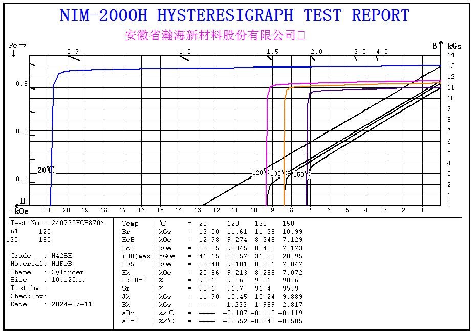
Hysteresis Loop Characteristics
The chart displays multiple closed curves representing the relationship between magnetic flux density (B) and magnetic field strength (H) at different temperatures (20°C, 120°C, 130°C, 150°C). These curves exhibit typical hysteresis loop shapes, reflecting energy loss and magnetic characteristics during magnetization and demagnetization processes.
Curve Interpretation
X-axis (H): Magnetic field strength in kOe (kilo-Oersteds), indicating external magnetic field magnitude
Y-axis (B): Magnetic flux density in kGs (kilo-Gauss), showing magnetization degree
Color-coded curves: Temperature-dependent hysteresis loops showing downward/leftward shifts with increasing temperature
Key Parameters and Significance
Remanence (Br)
Change: Decreases from ~13.00 kGs (20°C) to ~10.99 kGs (150°C)
Significance: Indicates reduced ability to retain magnetism at high temperatures, critical for high-temperature motor applications
Coercivity (Hcb)
Change: Drops from ~12.78 kOe (20°C) to ~7.129 kOe (150°C)
Significance: Shows decreased resistance to demagnetization at elevated temperatures, important for magnetic storage devices
Intrinsic Coercivity (Hcj)
Change: Gradually decreases with temperature
Significance: Reflects reduced domain structure stability under thermal stress, crucial for aerospace applications
Temperature Effects
Increasing temperature causes deterioration in Br, Hcb and Hcj due to intensified atomic thermal motion disrupting magnetic moment alignment. This impacts high-precision applications requiring stable performance.
Black Slope Lines Interpretation
These lines represent approximate linear magnetization behavior before saturation:
Slope significance: Indicates material permeability (μ)
Steeper slope = higher permeability (easier magnetization)
Shallower slope = lower permeability
Temperature impact: Slope changes demonstrate temperature’s effect on permeability
Practical importance: Critical for designing electromagnetic devices operating at various temperatures